Method of Calculating Temperature Rise in Self Cooled Transformers
Introduction
The modes of heat transfer in self-cooled transformers can be explained by simple thermodynamic concepts. The modes of transfer include convection, conduction, and radiation. Before one can understand how to calculate a temperature rise there must be a thorough understanding of these concepts.
The geometry of the coil has a great effect on the effectiveness of all modes of heat transfer. Along with the geometry the actual construction and materials used in a transformer have a great effect on its’ ability to cool.
One of the key factors in determining a temperature rise is an understanding of the actual losses in the device. The losses include I2R heating loss in the winding sometimes referred to as DC loss, skin effect loss, eddy loss, core loss, and stray loss of mechanical clamping components. Proper calculation of losses is absolutely critical to determine the actual temperature rise. This paper will not go into depth how to calculate losses. A general description of each is given with a either a formula, method for calculation, and possibly a reference for more information.
The concepts in this paper are imperative for a transformer design engineer to master. Specifying engineers can benefit from at least a cursory knowledge in order to ask the proper questions when specifying and purchasing components.
Discussion
Losses in a transformer
The losses in transformers can be attributed to three main categories these being winding loss, core loss and stray loss. Winding losses are broken up into DC loss, skin-effect loss and eddy loss. In order to have a background for temperature rise calculations a brief description of each follows.
DC loss is due to the in phase voltages and currents in the winding. Because the resistance is directly proportional to temperature so follows the DC loss. In order for a designer to have an accurate DC loss number there are several mechanical parameters that must be known including base resistivity of the winding material, conductor cross section, and the build of the windings in order to determine conductor length.
Wdc = (I2 R20) [(Kt + Tw)/(Kt + 20)] (W) (1)
Where: I = winding current (A)
R20 = resistance of winding at 20 °C
Kt = 234.5 for copper, 225 for aluminum
Tw = temperature of winding
Skin-effect is a measure of how much cross section of the wire current flows in. Skin-effect is dependent on frequency. If the frequency is great enough where this is a problem either multiples of a smaller wire are used or the cross section is decreased in the DC loss calculation. As a general rule of thumb equation (2) gives the skin depth for a given frequency in inches for a copper wire at 20°C. Before an engineer designs a part at any frequency above 400 Hz he should be familiar with the skin depth for the particular application. Ref [1] and [3] have very extensive treatments on the subject.
Dsk = 2.64 / f1/2 (in) (2)
Where: f = frequency (Hz)
The final component is eddy loss which is caused by non-uniform flux linkages across the width of the coil. Eddy loss (We) is created by currents transverse to real current flow. In the winding voltage fields are set-up by the magnetic flux not totally linking all turns of the winding. It is these fields which cause the eddy currents. Equation (3) will give eddy loss at any temperature. It should be noted that eddy loss is inversely proportional to temperature.
We = Ke[(f tk)2(NI/ww)2wLB][(Kt+75)/(Kt+Tw)](W) (3)
Where: Ke = 4 x 10⁻⁹ for copper
6.5 X 10⁻⁹ for aluminum
tk = wire thickness (in)
N = number of electrical turns
ww = winding width (in)
wLB = weight of wire (lb)
Eddy heating is a localized phenomena and not uniformly distributed across the coil. In order for a proper treatment of this, an analysis should be done using finite elements to determine the field shape. The method of temperature rise described here will treat the loss as it were uniformly distributed. The result will be a temperature distribution in the coil. A designer should keep this in mind and if in doubt should perform a well thermocoupled heat-run on a prototype unit. For anyone wishing to further investigate eddy loss Ref. [5] provides a very thorough treatise on the subject.
Core loss is due to the changing flux in the transformer core. Core loss is dependent on frequency, material, processing, induction level and core shape. Most designers use a curve provided by the steel manufacturer along with a destruction factor due to material degradation from handling and core geometry. Reference [6] provides a very thorough treatment on the material properties of electrical steels. Reference [5] has many formulas for different core geometries.
Stray loss is the loss in mechanical components due to magnetic flux linking them. This is rarely calculated in dry type units under 3000 KVA. It is only mentioned here for the sake of completeness.
Modes of heat transfer
Convection is one of the chief modes of heat loss in a transformer. In general the amount of convection is affected by difference in temperature between loss producing component and ambient, height of convective surface, surface quality of surface, and size of conductive channels. Formula (4) is the general form for convection from a large surface. Convection can take place on any surface of a transformer that has air passage over it.
Wc = 0.0014 P0.5 Tr1.25 (W/in2) (4)
Where: P = air pressure (atm)
Tr = temperature rise (°C)
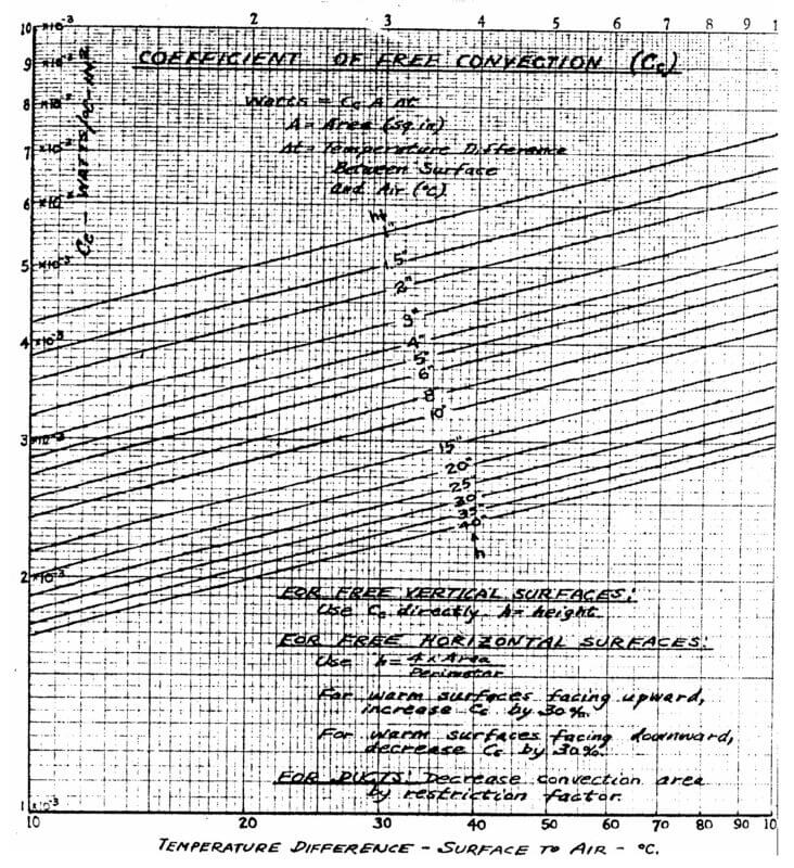
We will treat cooling by convection using the chart of figure 1 presented by Johnson [2]. This chart is based on free convection from vertical plates. For a horizontal surface facing up dissipation is 30% greater than the chart and for downward facing it is 30% less. Use formula (5) to determine the proper height curve for a vertical surface. The other factor to consider in convection cooling is the effectiveness of cooling channels. This is dependent on the height of the coil, thickness of channel and the amount of restrictions in the cooling channel. The author has found the rules of thumb in Table 1 apply for 100% effectiveness of the convection formulas provided the cooling channels are unobstructed.
hv = (4 A) / per (in) (5)
Where: A = area of plate (sq in)
per = perimeter of plate (in)
| Coil Height | Channel Thickness |
| Up to 6” | 3/8” |
| 6 – 18” | ½” |
| 18 – 30” | 5/8” |
| 30 – 48” | ¾” |
Table 1: Cooling Channel Sizes
In order to read a number from figure 1 you need to determine the height of the convective surface, which would normally be the electrical height of a coil for a vertical surface or calculated using formula (5) for a horizontal surface. Also the temperature rise must be known. This may seem ambiguous because we are trying to calculate the temperature rise but this is an iterative process where an initial guess is used and the calculated rise is used for the next iteration. Formula (6) shows how to calculate temperature rise using the chart and assuming only convection cooling of a surface.
Trc = Lossc / (Kc Ac) (°C ) (6)
Where: Lossc = Total loss from surface (W)
Kc = coefficient (W/°C in2)
Ac = convection area (in2)
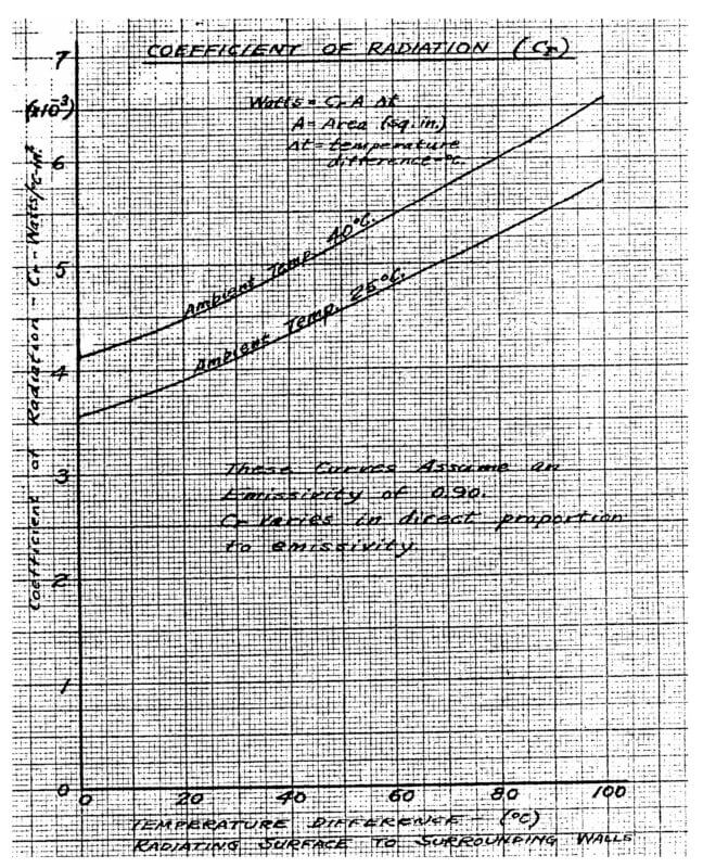
Radiation is the other main vehicle for heat dissipation in a transformer. Radiation is governed by the Stefan-Boltzman Law Equation (7). Factors affecting radiation include differential of temperature between air and the heated object and the emissivity factor which is due to surface factors including roughness and color. Reference [7] describes various surface treatments and colors as to their effectiveness for emissivities. Radiation takes place on surfaces that are directly exposed to ambient air. Generally the only surfaces in a transformer effective for radiation would be the outer coil surfaces not in the window area and the exposed edges of the core laminations.
Wr = 36.6 X 10⁻¹² E (TO4 –TA4) (W/in2) (7)
Where: E = emissivity factor
TO = temperature of object (K)
TA = temperature of ambient (K)
Radiation will be calculated using Formula (8) which is a curve fit of Figure 2 from Johnson [2]. An emissivity factor of 0.90 will be assumed. If a particular design has a different emissivity this equation can be prorated.
Trr = Lossr / (Kr Ar) (°C ) (8)
Where: Lossr = Total loss from surface (W)
Kr = coefficient (W/°C in2)
Ar = radiation area (in2)
Conduction is treated more as a mode of moving loss from one area to another rather than true dissipation. Depending on transformer design loss can be transferred between windings and the core. In the model this loss must still be dissipated to the air in some manner. Conduction also comes into play in dealing with insulation materials. Because insulations have such low thermal conductivity compared to metals they really hamper a coils ability to cool. These types of conductive transfers will essentially cause a higher average rise in temperature. Conduction is also what causes hot-spot temperatures in a winding. Equation 9 is the general form for temperature rise due to conduction. Constant (k) is dependent on material and temperature.
∆Tcd = Q (Lcd / k Acd) (°C ) (9)
Where: Q = Heat loss (W)
Lcd = Length of conduction (in)
k = constant ((W/in K)
Acd = cross section of material (in2)
Discussion of modeling transformer windings
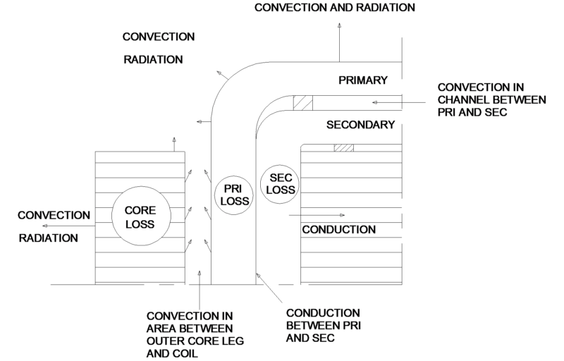
Three distinct types of core and coil models will be discussed. They include un-ducted coils, coils with vertical cooling channels where there is conduction between windings (End Ducted), and vertical cooling channels with no conduction between windings (Full Ducted). Figure 3 shows a generic drawing for a transformer and points out the surfaces useful for convection and conduction in an un-ducted design.

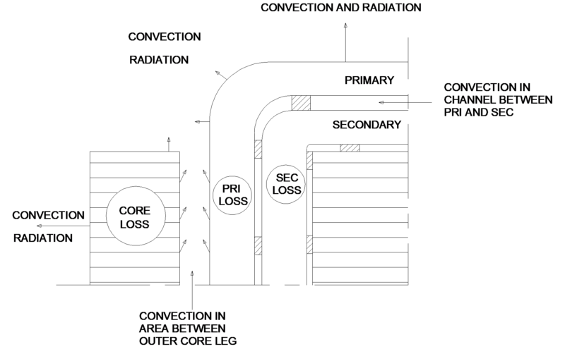
The first type, un-ducted, is the simplest method. In this type all loss is added together and all exposed areas are useful radiation and convection. When calculating areas of convection keep in mind the correction factors for horizontal and vertical surfaces and treat these as effective areas. The designer also needs to understand how the unit will be mounted as this will change the effectiveness of the convection surfaces. Figure 4 is a cross section of an un-ducted design and the arrows show major paths of heat flow. This method will give a single temperature rise. The designer must pay attention to actual construction to insure the effectiveness of actual conduction paths as opposed to his calculated numbers.

The next model is one in which there is an end duct between primary and secondary and the coil does not touch the outer leg. This model is more complicated because the loss must be broken up into different parts which are dissipated from a particular surface. Since we are most concerned with coil temperature rise the actual rise of the core will not be calculated. In this model approximately half of the core loss of the center leg will need to be dissipated thru coil surfaces.
The final distinct model is called full ducted. In this design there is little to no conduction between core and sections of the winding. Figure 6 shows areas for consideration in modeling. In this model two temperature rises will be calculated for the coil.
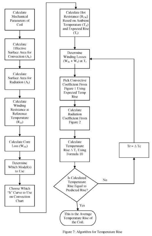
Development of an algorithm
Figure 7 summarizes an algorithm which ties together all the items discussed previously. The author has implemented this algorithm in an Excel spreadsheet along with Visual Basic routines for some iterative and repetitious functions. Properly implemented this is a relatively easy way to predict the temperature rise of a coil given the physical parameters. A combination of equations (6) and (8) is shown in equation (10). This equation will be used for the iterative calculation in the algorithm.
∆Tc = Loss / ((Kr Ar) + (Kc Ac)) (°C ) (10)
Where: Loss = Total loss from surface (W)
Conclusions
This paper has presented numerous concepts and formulas for use in the calculation of temperature rise for transformers. Most information is not new, in fact many of the reference texts cited are 50+ years old. In spite of this fact the information is based on the laws of Physics and has not changed. I strongly recommend all engineers involved with the design of transformers to seek out the reference texts listed.
The three models listed here were chosen since they are the most common in practice. Using the basic formulas presented and the algorithm a designer should be able to model his particular design. No discussion of forced cooling was given but this can very easily be implemented.
I welcome further discussion on this subject. With the number of finite element software packages available a more refined treatment of losses and hot spot temperatures is possible.
References:
- Dwight, Herbert Bristol. Electrical Coils and Conductors, McGraw-Hill, 1945,
- Johnson, Walter C. Calculation of the Temperature rise of Air-Cooled Transformers, The Pennsylvania State College Department of Electrical Engineering, June 1942.
- McLyman, Colonel Wm. T. Transformer and Inductor Handbook, Marcel Dekker, Inc., 1988.
- Principles of inductor Design, Optimized Program Service, Inc. O. Box 425, Berea, Oh 44017, 1987.
- Karsai, K., Kerényi, D., Kiss, L., Large Power Transformers, Elsevier, 1987.
- Bozorth, Richard M. Ferromagnetism, D. Van Nostrand Company, Inc. 1951.
- Blume, L.F., Camilli, G., Boyajian, A., Montsinger, V.M., Transformer Engineering, John Wiley & Sons, Inc. 1938.
- Schmidt, Frank W., Henderson, Robert E., Wolgemuth, Carl H., Introduction to Thermal Sciences, John Wiley & Sons, 1984.